
Coverage Technical Report, Census of Population, 2016
8. Census Overcoverage Study (COS)
8.1 Overview and methodology
Prior to 2006, the level of overcoverage caused by duplication of individuals on the census was measured by three studies, each one covering part of the overcoverage: the Automated Match Study (AMS), the Collective Dwelling Study (CDS) and the Reverse Record Check (RRC). Since 2006, given and family names have been included in the Census Response Database,Note 1 and overcoverage is now measured with a single study: the Census Overcoverage Study (COS). Hence, the RRC is no longer used to measure overcoverage, and the CDS was discontinued. The AMS is still conducted for evaluation purposes.
As was the case with both the 2006 and 2011 overcoverage studies, the 2016 COS was based on a series of probabilistic record linkage operations and manual verification of pairs of potential overcoverage cases. These record linkage operations also involved the use of certain administrative data files.
For ease of reference, in the rest of this section, a pair of potential overcoverage cases is referred to as a pair, and a pair that has been confirmed to be the same person is referred to as a duplicate.
The 2016 COS was a statistical study in which overcoverage was estimated with a probabilistic sample selected from a frame of potential overcoverage cases. The COS involves all the steps one would find in a statistical survey:
- sampling frame construction
- sample selection
- data collection
- processing and verification of collected data
- weighting and estimation
- analysis.
However, the COS differs from a statistical survey in the following ways:
- The sampling frame was constructed by means of successive probabilistic and deterministic record linkage operations.
- Collection was based on manual verification of sampled pairs of records and did not involve respondents.
The COS methodology for estimating 2016 overcoverage was based on matching persons without geographic restrictions, while the AMSNote 2 was based on matching private households located in the same geographic area. The 2016 COS took advantage of the fact that the 2016 Census Response Database (RDB) contains respondents’ surnames and given names in two separate variables. This made it possible to produce a more precise estimate of the overcoverage caused by persons enumerated more than once on the census database. The COS used automated matching and manual verification methods. It included individuals living in collective dwellings and did not impose geographic restrictions such as those imposed on the AMS.
The census database used for the COS was the same as the database used for the RRC: the CCS-RDB. For simplicity, it is hereby referred to as the RDB.
As in 2006 and 2011, the 2016 COS sampling frame was constructed in multiple steps. The first step was an internal probabilistic record linkage in which the entire RDB was linked to itself. The second step was an external probabilistic record linkage in which the entire RDB was linked to an administrative frame (ADMIN) built from the Canadian Statistical Demographic Database (CSDD). The CSDD is an administrative database created from multiple administrative data sources for use in the Census Program.
The two probabilistic linkages were conducted with G-Link 3.2, the probabilistic record linkage system designed at Statistics Canada that uses the Fellegi-Sunter method to solve large file linkage problems when there are no direct identifiers common to both sources (Fellegi and Sunter 1969).
8.2 Construction of the sampling frame
The COS began with the construction of a sampling frame of potential overcoverage cases using probabilistic and deterministic record linkage. This work consisted of the following four steps:
- probabilistic record linkage between the RDB and itself
- probabilistic record linkage between the RDB and the ADMIN
- extension of the sampling frame based on households
- supplement frame: additional potential overcoverage identified during evaluation of CSDD prototype.
8.2.1 Input files for the construction of the COS sampling frame
The RDB contained a little under 34 million records and included responses from individuals living in both private and collective dwellings. It contained names (including given names and surnames), demography (including date of birth and sex) and geography (including province or territory and postal code). The ADMIN was extracted from the CSDD and contained over 48 million records. As in 2011, the ADMIN included names (given name and surname), demographic information (including date of birth and sex) and geographic information (including province or territory and postal code).
The CSDD from which the ADMIN is drawn was built using multiple administrative data files. These included tax files provided by the Canada Revenue Agency; immigrant and non-permanent resident files provided by Immigration, Refugees and Citizenship Canada; birth records from vital statistics files provided by Vital Statistics; the National Routing System; and the Indian Registry, provided by Indigenous and Northern Affairs Canada.
The records of persons classified as living in one of the three territories according to the CSDD were replaced by the information from territorial health care files used as a sampling frame for the RRC, as these were believed to provide better coverage of individuals living in the territories.
The following matching variables were used in both the RDB-to-RDB linkage and the RDB-to-ADMIN linkage:
- names: given name and surname variables
- demographic data: date-of-birth and sex variables
- geographic data: province or territory and postal code variables.
8.2.2 Steps in constructing the COS frame
The COS frame included all pairs forming potential overcoverage cases that were outputted by G-Link following steps 1 and 2, and those identified by the extension. It also included record pairs identified by the supplement. Construction of the COS frame is illustrated in Figure 8.2.2 below:
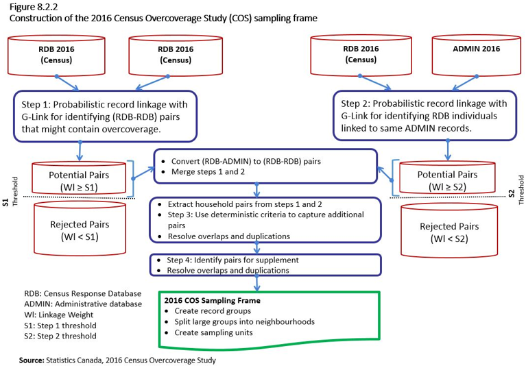
Description for Figure 8.2.2
The title of Figure 8.2.2 is “Construction of the 2016 Census Overcoverage Study (COS) sampling frame.”
The first text box in this figure contains Step 1, probabilistic record linkage with G-Link for identifying (RDB-RDB) pairs (i.e., 2016 Census Response Database [RDB] and 2016 Census Response Database pairs) that might contain overcoverage.
This text box points to two types of pairs: potential pairs (linkage weight greater than or equal to the Step 1 threshold) and rejected pairs (linkage weight less than the Step 1 threshold).
Potential pairs are shown above the upper Step 1 threshold.
On the other side of the figure is a text box that contains Step 2, probabilistic record linkage with G-Link for identifying RDB individuals linked to the same administrative database (ADMIN) records.
This text box points to two types of pairs: potential pairs (linkage weight greater than or equal to the Step 2 threshold) and rejected pairs (linkage weight less than the Step 2 threshold).
Potential pairs are shown above the upper Step 2 threshold.
The left-hand side box that contains potential pairs from Step 1 and the right-hand side box that contains potential pairs from Step 2 both point to the next text box, which is in the middle of the figure and contains the following two bullets:
- Convert the (RDB-ADMIN) to (RDB-RDB) pairs.
- Merge Step 1 and Step 2.
An arrow points down to the next text box, which contains three bullets:
- Extract household pairs from steps 1 and 2.
- Step 3: Use deterministic criteria to capture additional pairs.
- Resolve overlaps and duplications.
Beneath that text box is another text box, which contains the following two bullets:
- Step 4: Identify pairs for supplement.
- Resolve overlaps and duplications.
Beneath that text box is an arrow that points to the final text box, 2016 COS Sampling Frame, which contains three bullets:
- Create record groups.
- Split large groups into neighbourhoods.
- Create sampling units.
Source: Statistics Canada, 2016 Census Overcoverage Study
8.2.3 Step 1: Probabilistic RDB-RDB linkage
The purpose of Step 1 was to measure overcoverage in persons on the RDB. To optimize the record linkage, provincial and territorial name frequency classes were created to compare the given names and surnames. The name frequency classes were used as outcome levels in the concordance rules for names in G-Link 3.2.
This linkage process was based on the following series of operations:
- Create RDB-RDB potential pairs by applying selection criteria.
- Compute name frequencies (for family names and given names) within each province and territory.
- Create name frequency classes.
- Compare the records for the potential pairs by applying concordance rules.
- Calculate the weights of the results of the rule application using the EM algorithm.
- Calculate provincial and territorial thresholds.
- Select pairs whose weight was greater than the thresholds.
From Step 1, a linked set of 4,254,360 potential pairs was created.
8.2.4 Step 2: Probabilistic RDB-ADMIN linkage
The purpose of Step 2 was to identify additional potential overcoverage not captured by the Step 1 linkage. RDB record pairs were created from groups of multiple RDB records linked to the same ADMIN record. This matching process identified pairs where the errors in the names or date of birth were such that the RDB-RDB linkage was not able to match them when they were compared directly. It also picked out pseudo-duplicates, which were RDB and ADMIN records that shared many match variables with a high linkage weight, but actually represented different individuals. For this reason, a clean-up of the RDB-RDB pairs derived from the RDB-ADMIN pairs was performed.
Step 2 involved the following sequence of operations:
- Create RDB-ADMIN potential pairs by applying selection criteria.
- Compute name frequencies within each province and territory.
- Create name frequency classes.
- Compare the records for the potential pairs by applying concordance rules.
- Calculate the weights of the results of the rule application using the EM algorithm.
- Calculate the provincial and territorial thresholds.
- Select pairs whose weight was greater than the threshold.
- Create RDB-RDB pairs from the set of RDB-ADMIN pairs above the thresholds.
- Remove pairs already identified with the Step 1 linkage.
- Verify and clean up the RDB-RDB pairs derived from RDB-ADMIN pairs to reduce the pseudo-duplicates.
The RDB-ADMIN linkage identified 930,120 additional pairs that were added to the set of potential pairs.
8.2.5 Step 3: Extension of the sampling frame based on households
The purpose of extending the sampling frame was to find additional overcoverage in households that contained potential overcoverage cases from Step 1 or Step 2. This phase resulted in the creation of additional RDB-RDB record pairs, which were produced in two steps.
First, a household pair was produced for each RDB-RDB person pair created in Step 1 or Step 2 by adding the other household members to it. Second, using sex and date of birth as variables, new RDB-RDB pairs were identified by comparing the persons present in the household pair. Comparison rules were applied to identify pairs that might represent overcoverage cases. The frame extension included pairs from two private households, or pairs where an individual from a private household was linked to an individual from a collective. Pairs where both records were from collectives were excluded.
As was done with the RDB-ADMIN pairs, pairs already identified in the first two steps were removed. When the duplicates were removed, the extension frame captured a further 167,980 pairs, which were added to the set of potential pairs.
8.2.6 Creation of the sampling units
Potential overcoverage cases were identified using groups of interconnected RDB records. The RDB-RDB person pairs returned by steps 1 and 2, and the extension, were pooled. Mutually exclusive record groups were created from the set of unduplicated person pairs, meaning that a record group contained all the RDB records connected by potential overcoverage, as identified in steps 1 to 3. For cases where the record groups contained more than 10 RDB records, a graph theory method was applied to reduce the group into small subgroups called “neighbourhoods” to facilitate manual verification.
8.2.7 Step 4: Supplement frame
During the evaluation of the 2016 CSDD prototype, the CSDD team identified potential duplicates in the RDB. Their list of potential duplicates was compared with the COS sampling frame constructed from steps 1 to 3. Most of the potential pairs identified by the CSDD team had been captured in the first three steps described above. However, some of these pairs were found to be missing from the set of potential pairs created with the first three steps. An investigation of the missing pairs found a few additional pairs not identified by the CSDD team that should have been included in the set of potential pairs. A total of 97,000 pairs were identified in this manner and were added to the COS sampling frame.
The final COS sampling frame contained a little over 3.6 million sampling units, created from approximately 5.4 million RDB-RDB pairs.
8.3 Census Overcoverage Study sample design
To meet sampling requirements, the sampling frame units were separated into four strata:
- Stratum 1: This consists of the intraprovincial units from steps 1 to 3. These are the sampling units created during steps 1 to 3 where all the RDB records that formed the pairs in the unit were in the same province or territory.
- Stratum 2: This consists of the interprovincial pairs from steps 1 to 3. These are the sampling units created during steps 1 to 3 and formed from a single pair of records from two different provinces or territories.
- Stratum 3: This consists of the interprovincial groups and neighbourhoods from steps 1 to 3. These are the sampling units created during steps 1 to 3 and formed from at least two pairs of records, covering at least two different provinces or territories. It should be noted that such a unit could contain intraprovincial pairs. For example, a group could be composed of three pairs linking RDB records in Ontario, and another pair linking an Ontario record with an Alberta record.
- Stratum 4: This consists of the pairs from Step 4. These are pairs of potential duplicates determined by the supplement. This stratum included both intraprovincial and interprovincial pairs.
8.3.1 Sample allocation
The 2016 COS manual verification budget was based on a total sample size similar to the one used in 2011—i.e., a total sample of 54,000 pairs to verify for strata 1 to 3. It was decided that, on average, 70% of a province’s sample would be intraprovincial pairs, and the rest would be interprovincial pairs. This represented a reduction in the proportion of intraprovincial pairs in the sample (which was approximately 80% in 2011), given that the 2016 frame contained more interprovincial pairs.
The sample of pairs was divided between the provinces and territories using a power allocation method, with the total number of pairs in the frame for each province and territory as its size, and = 0.2 as its power. This made it possible to obtain precise estimates for each province, and nationally, while allowing for a sample distribution that was not too different from that of 2011. The next step involved distributing the provincial and territorial sample between the intraprovincial and interprovincial pairs. As mentioned, the ideal overall proportion was for 70% of each provincial sample to be intraprovincial pairs. A smaller proportion was used for Prince Edward Island and the three territories since the 2011 results showed that the contribution of interprovincial overcoverage was larger there. Inversely, a higher proportion was used for Quebec, Ontario and British Columbia. The same proportion was then used in the other provinces and was set to obtain the national proportion of 70%.
Once the sample size of intraprovincial and interprovincial pairs was determined for each province and territory, the next step was to divide these samples between the three strata. The sample of interprovincial pairs was separated between strata 2 and 3 based on the proportion of interprovincial pairs from the frame in each of the two strata. It was not possible to allocate the sample of intraprovincial pairs between strata 1 and 3 in the same manner. In fact, in stratum 3, the groups and neighbourhoods were composed mainly of interprovincial pairs, so selecting the desired number of intraprovincial pairs would have resulted in too many interprovincial pairs being selected. To avoid this problem, simulations showed that 85% of the sample of intraprovincial pairs had to be selected from stratum 1 to make the sample from stratum 3 usable. For Prince Edward Island and the three territories, it was practically a take-all. All the pairs from the stratum 1 frame were therefore selected there.
For stratum 4, the sample size was set at 3,000 pairs, based on the desired level of precision, available resources and the schedules to be met when the pairs from the supplement frame were determined.
8.3.2 Sample from stratum 1
Stratum 1 was separated into three substrata within each province: pairs, groups and neighbourhoods. An optimal sample allocation based on manual verification costs was used to allocate the provincial sample of this stratum to substrata. A systematic sample of pairs sorted by linkage weight class, age group, sex, marital status, mother tongue and CMA was then selected. For groups and neighbourhoods, a simple random sample was selected. Table 8.3.2 provides the distribution of sampling units from stratum 1 in the sampling frame and in the sample for each province and territory.
| Provinces and territories | Frame totals | Sample totals | ||||||
|---|---|---|---|---|---|---|---|---|
| Pairs | Groups | Neighbourhoods | Total | Pairs | Groups | Neighbourhoods | Total | |
| Canada | 1,165,224 | 192,530 | 172,610 | 1,530,364 | 30,481 | 1,702 | 1,420 | 33,603 |
| Newfoundland and Labrador | 9,133 | 296 | 159 | 9,588 | 2,386 | 96 | 74 | 2,556 |
| Prince Edward Island | 1,763 | 42 | 20 | 1,825 | 1,763 | 42 | 20 | 1,825 |
| Nova Scotia | 14,328 | 626 | 368 | 15,322 | 2,644 | 137 | 82 | 2,863 |
| New Brunswick | 13,844 | 591 | 309 | 14,744 | 2,604 | 129 | 60 | 2,793 |
| Quebec | 413,625 | 102,703 | 76,085 | 592,413 | 3,284 | 416 | 308 | 4,008 |
| Ontario | 479,444 | 71,845 | 82,517 | 633,806 | 3,947 | 295 | 392 | 4,634 |
| Manitoba | 18,440 | 835 | 512 | 19,787 | 2,724 | 107 | 76 | 2,907 |
| Saskatchewan | 17,175 | 833 | 415 | 18,423 | 2,532 | 118 | 53 | 2,703 |
| Alberta | 75,638 | 4,261 | 3,448 | 83,347 | 3,445 | 126 | 118 | 3,689 |
| British Columbia | 120,458 | 10,460 | 8,775 | 139,693 | 3,776 | 198 | 235 | 4,209 |
| Yukon | 570 | 16 | 2 | 588 | 570 | 16 | 2 | 588 |
| Northwest Territories | 345 | 8 | 0 | 353 | 345 | 8 | 0 | 353 |
| Nunavut | 461 | 14 | 0 | 475 | 461 | 14 | 0 | 475 |
| Source: Statistics Canada, 2016 Census Overcoverage Study. | ||||||||
8.3.3 Sample from stratum 2
Sampling units from stratum 2 were all interprovincial pairs. Stratum 2 was therefore subdivided based on the province of the pair’s two CCS-RDB records. The pairs for a combination of province 1 and province 2 were then sorted according to the same variables used in stratum 1, and a systematic sample was selected. Table 8.3.3 provides the distribution of the sampling units from stratum 2 in the sampling frame and the sample for each province and territory. It must be noted that because each pair belongs to two different provinces, the sum of the number of pairs in each province and territory corresponds to twice the number of pairs at the national level, since the pairs are counted in two places.
| Provinces and territories | Pairs on the frame | Pairs in the sample |
|---|---|---|
| Canada | 1,029,616 | 3,658 |
| Newfoundland and Labrador | 52,174 | 640 |
| Prince Edward Island | 15,546 | 561 |
| Nova Scotia | 93,331 | 695 |
| New Brunswick | 77,998 | 650 |
| Quebec | 316,352 | 490 |
| Ontario | 670,953 | 580 |
| Manitoba | 99,259 | 665 |
| Saskatchewan | 83,571 | 655 |
| Alberta | 293,933 | 495 |
| British Columbia | 348,355 | 500 |
| Yukon | 3,070 | 466 |
| Northwest Territories | 3,147 | 513 |
| Nunavut | 1,543 | 406 |
| Source: Statistics Canada, 2016 Census Overcoverage Study. | ||
8.3.4 Sample from stratum 3
Stratum 3 was composed of interprovincial groups and neighbourhoods. As previously mentioned, a large number of these sampling units contained intraprovincial pairs. The challenge was therefore to select enough intraprovincial pairs, especially for the small provinces and the territories, without selecting too many interprovincial pairs or pairs of units in the large provinces. To do this, units from stratum 3 were divided in the following manner, using dominance rules based on the proportion of intraprovincial pairs belonging to the same province within interprovincial groups and neighbourhoods:
- units where at least 60% of the pairs were intraprovincial for a given province
- units where between 50% and 60% of the pairs were intraprovincial for a given province
- units where less than 50% of the pairs belonged to the same province.
A simulation was conducted to determine the sample size required in each substratum to obtain the targeted sample sizes for the number of intraprovincial and interprovincial pairs in each province. A simple random sample of groups and neighbourhoods was selected in each substratum. For each substratum, Table 8.3.4 presents the dominance rule applied (most frequent proportion and province), the number of sampling units (groups and neighbourhoods) in the substratum, the number of pairs making up these units, and the number of units sampled.
Substrata 1 to 11 were composed of sampling units where at least 60% of intraprovincial pairs were found in the same province or territory (there were none in Yukon or Nunavut). Substrata 13 to 16 were formed from units composed of interprovincial pairs only, and where the most frequent province or territory among all the CCS-RDB records in the unit were respectively Prince Edward Island (9911), Yukon (9960), the Northwest Territories (9961) or Nunavut (9962). Substratum 12 contained all the other units composed of interprovincial pairs only. Substrata 17 to 29 were composed of units where at least 50%, but less than 60%, of intraprovincial pairs came from a given province. Finally, substrata 30 to 42 included all the other sampling units, classified according to the most frequent province among all the intraprovincial pairs. For example, substratum 23 was composed of all units where at least 50%, but less than 60%, of intraprovincial pairs came from Manitoba.
| Substratum | Province or territory | Number of sampling units on the frame | Number of pairs in the sampling units | Number of sampled units |
|---|---|---|---|---|
| Total | Canada | 997,209 | 3,113,046 | 3,766 |
| 60% or more | ||||
| 1 | 10 | 98 | 374 | 98 |
| 2 | 11 | 16 | 56 | 16 |
| 3 | 12 | 261 | 982 | 168 |
| 4 | 13 | 234 | 1,008 | 139 |
| 5 | 24 | 35,259 | 157,968 | 237 |
| 6 | 35 | 56,977 | 250,169 | 236 |
| 7 | 46 | 208 | 837 | 148 |
| 8 | 47 | 168 | 762 | 117 |
| 9 | 48 | 2,108 | 8,465 | 185 |
| 10 | 59 | 8,986 | 37,667 | 214 |
| 11 | 61 | 1 | 3 | 1 |
| 12 | 9900 | 424,804 | 971,198 | 275 |
| 13 | 9911 | 10,664 | 28,813 | 81 |
| 14 | 9960 | 1,974 | 5,310 | 81 |
| 15 | 9961 | 1,988 | 5,329 | 81 |
| 16 | 9962 | 681 | 1,911 | 81 |
| At least 50% but less than 60% | ||||
| 17 | 10 | 1,057 | 2,314 | 152 |
| 18 | 11 | 174 | 381 | 102 |
| 19 | 12 | 2,175 | 4,773 | 60 |
| 20 | 13 | 1,614 | 3,667 | 60 |
| 21 | 24 | 44,438 | 114,348 | 78 |
| 22 | 35 | 112,607 | 301,663 | 97 |
| 23 | 46 | 1,731 | 3,790 | 95 |
| 24 | 47 | 1,262 | 2,784 | 95 |
| 25 | 48 | 12,287 | 28,069 | 129 |
| 26 | 59 | 27,016 | 69,808 | 119 |
| 27 | 60 | 22 | 44 | 22 |
| 28 | 61 | 8 | 16 | 8 |
| 29 | 62 | 5 | 10 | 5 |
| Less than 50% | ||||
| 30 | 10 | 2,335 | 9,959 | 64 |
| 31 | 11 | 378 | 1,544 | 75 |
| 32 | 12 | 4,461 | 18,969 | 44 |
| 33 | 13 | 3,783 | 15,606 | 44 |
| 34 | 24 | 38,148 | 162,831 | 30 |
| 35 | 35 | 96,087 | 422,284 | 30 |
| 36 | 46 | 3,903 | 17,103 | 44 |
| 37 | 47 | 3,089 | 13,033 | 44 |
| 38 | 48 | 22,495 | 101,325 | 30 |
| 39 | 59 | 73,556 | 347,254 | 30 |
| 40 | 60 | 80 | 322 | 80 |
| 41 | 61 | 55 | 230 | 55 |
| 42 | 62 | 16 | 67 | 16 |
| Source: Statistics Canada, 2016 Census Overcoverage Study. | ||||
8.3.5 Sample from stratum 4
Stratum 4 contained all the record pairs determined using the supplement. Since stratum 4 was added after the groups and neighbourhoods formed by the interconnected pairs from steps 1 to 3 were created, all the sampling units from stratum 4 were treated as pairs. This stratum was substratified by province. A power allocation was used to allocate the sample of 3,000 pairs between the provinces and territories. Also, an optimal allocation, based on the expected overcoverage rates, made it possible to allocate one province’s sample between the intraprovincial and interprovincial pairs. A systematic sample of pairs from the RDB was then chosen in each substratum. For each province and territory, Table 8.3.5 presents the total number of intraprovincial and interprovincial pairs in the frame, and the number of pairs sampled. As mentioned, it is important to note that, for interprovincial pairs, the national-level total corresponds to half the sum of the numbers from each province and territory since each interprovincial pair is counted in total in two provinces.
| Provinces and territories | Pairs on the frame | Pairs in the sample | ||
|---|---|---|---|---|
| Intraprovincial | Interprovincial | Intraprovincial | Interprovincial | |
| Canada | 74,987 | 22,099 | 2,520 | 548 |
| Newfoundland and Labrador | 967 | 935 | 144 | 70 |
| Prince Edward Island | 221 | 314 | 87 | 61 |
| Nova Scotia | 1,608 | 1,836 | 163 | 93 |
| New Brunswick | 1,314 | 1,377 | 156 | 81 |
| Quebec | 15,803 | 5,922 | 367 | 95 |
| Ontario | 31,264 | 13,927 | 444 | 128 |
| Manitoba | 2,109 | 2,427 | 177 | 101 |
| Saskatchewan | 1,886 | 2,192 | 170 | 99 |
| Alberta | 7,831 | 6,982 | 272 | 122 |
| British Columbia | 11,763 | 7,979 | 319 | 116 |
| Yukon | 78 | 81 | 78 | 34 |
| Northwest Territories | 56 | 113 | 56 | 53 |
| Nunavut | 87 | 113 | 87 | 43 |
| Source: Statistics Canada, 2016 Census Overcoverage Study. | ||||
8.4 Collection
The collection process involved manually verifying the samples of selected pair groups. Manual verification was done pair by pair. When a group or neighbourhood was sampled, all the pairs it contained were examined manually. The pairs were examined only once, even if they belonged to more than one sampled neighbourhood.
The manual verification process involved an exhaustive review of all of the information available on the CCS-RDB. As in 2011, it included the following steps:
- comparing persons sampled from the CCS-RDB by name, sex, birth date and relationships between persons
- comparing members of households in the CCS-RDB according to the same criteria
- evaluating evidence for or against overcoverage between the two persons in the pair to determine whether the two records actually represent the same person
- determining the overcoverage scenario, coded only when there was verified overcoverage between non-identical households. Overcoverage scenarios are provided in Table 8.4.
| Code | Overcoverage scenario between non-identical households |
|---|---|
| 1.1 | Student or young adult newly away from home |
| 1.2 | Young adult newly away from home because of marriage or common-law relationship |
| 1.3 | Adult entering into or leaving married or common-law relationship |
| 2.1 | Child or children of parents in separate households |
| 2.2 | Child or children with two relatives or adults |
| 3.1 | Adult with other relatives |
| 3.2 | Adult with other unrelated adults |
| 4.1 | Collective dwelling |
| 5.1 | Other |
| Source: Statistics Canada, 2016 Census Overcoverage Study. | |
The manual verification sample was divided into batches of 150 pairs. One batch was entirely verified by the same coder. Once a batch was verified, it was evaluated using a statistical quality control operation.
8.5 Weighting and estimation
The starting weight of a sampling unit was simply the inverse of its probability of being selected. Given that the sampling units composed of groups or neighbourhoods varied with respect to the number of pairs they contained, a calibration step was added to ensure a good representation of the number of pairs in each province and territory. In stratum 1 (intraprovincial units), the sampling weights were calibrated so the estimated number of pairs corresponded to the total number of pairs in the frame for each province and territory. In stratum 3 (interprovincial groups and neighbourhoods), the sampling weights were calibrated so the estimated number of intraprovincial and interprovincial pairs in each province and territory was equal to the corresponding total from the frame. Thus, 13 control totals were used for stratum 1, compared with 26 for stratum 3. Statistics Canada’s Generalized Estimation System (G-Est) was used for the calibration. No calibration was required for strata 2 and 4, since they contained only pairs. Table 8.5a presents the three calibration factors for each province and territory.
| Provinces and territories | Stratum 1 | Stratum 3 | |
|---|---|---|---|
| Intraprovincial | Interprovincial | ||
| Newfoundland and Labrador | 1.003 | 1.049 | 0.899 |
| Prince Edward Island | 1.000 | 1.057 | 1.136 |
| Nova Scotia | 0.998 | 1.071 | 0.945 |
| New Brunswick | 0.996 | 0.901 | 1.225 |
| Quebec | 1.013 | 0.988 | 0.942 |
| Ontario | 1.014 | 1.001 | 1.008 |
| Manitoba | 1.008 | 1.013 | 1.117 |
| Saskatchewan | 1.007 | 1.041 | 0.962 |
| Alberta | 1.000 | 0.971 | 0.997 |
| British Columbia | 0.999 | 0.956 | 0.951 |
| Yukon | 1.000 | 1.039 | 1.415 |
| Northwest Territories | 1.000 | 1.015 | 1.468 |
| Nunavut | 1.000 | 1.000 | 0.493 |
| Source: Statistics Canada, 2016 Census Overcoverage Study. | |||
The results of the manual verification were processed to create overcoverage groups for estimation. Overcoverage groups were formed from all the RDB records linked by verified overcoverage. The COS estimates were obtained by adding the estimated overcoverage counted in each overcoverage group. For an overcoverage group that was a simple pair, the overcoverage count was 1. If the overcoverage group was contained in a small group of records (i.e., a group that had not been split into neighbourhoods), then the following formula was applied:
Overcoverage = number of records in the overcoverage group - 1.
For overcoverage groups split into neighbourhoods, overcoverage was counted according to the following two steps:
- calculating the overcoverage in each neighbourhood for which the anchor (i.e., the CCS-RDB record serving as the centre of the neighbourhood) was involved in verified overcoverage cases for this overcoverage group, as follows:
- Overcoverage in the neighbourhood =
- adding the overcoverage of each neighbourhood to obtain the total overcoverage of the group.
Overcoverage for a domain was obtained by multiplying the total overcoverage of the pair, group or neighbourhood by the proportion of CCS-RDB records that were part of the domain among those that belonged to the overcoverage group.
In all the cases described above, the overcoverage calculated for a unit was multiplied by the sampling unit’s post-calibration weight to obtain the weighted estimation. The variance was estimated with G-Est, which uses Taylor linearization.
Similar to what was done in the 2006 and 2011 COS, an adjustment based on the AMS was applied to the COS estimates to take into account the overcoverage measured by the AMS outside the COS universe. The adjustment factor was calculated and applied separately for each province and territory. The final variance took this adjustment into account. Table 8.5b shows the adjustment factor applied for each province and territory, for the last three iterations of the COS.
| Provinces and territories | 2006 | 2011 | 2016 |
|---|---|---|---|
| Newfoundland and Labrador | 1.029 | 1.030 | 1.035 |
| Prince Edward Island | 1.028 | 1.017 | 1.003 |
| Nova Scotia | 1.034 | 1.021 | 1.012 |
| New Brunswick | 1.040 | 1.071 | 1.037 |
| Quebec | 1.026 | 1.016 | 1.008 |
| Ontario | 1.040 | 1.020 | 1.015 |
| Manitoba | 1.035 | 1.025 | 1.010 |
| Saskatchewan | 1.039 | 1.010 | 1.006 |
| Alberta | 1.058 | 1.018 | 1.026 |
| British Columbia | 1.037 | 1.017 | 1.029 |
| Yukon | 1.027 | 1.014 | 1.010 |
| Northwest Territories | 1.039 | 1.169 | 1.015 |
| Nunavut | 1.061 | 1.015 | 1.023 |
|
AMS: Automated Match Study. COS: Census Overcoverage Study. Sources: Statistics Canada, 2006, 2011 and 2016 Census Overcoverage Study. |
|||
8.6 Final results
8.6.1 Overcoverage by step
The contribution of each step, and of the AMS adjustment, to the 2016 COS overcoverage estimates is provided in Table 8.6.1.
| Provinces and territories | Step 1 | Step 2 | Step 3 | Step 4 | AMS adjustment | |||||
|---|---|---|---|---|---|---|---|---|---|---|
| Estimated number | Percentage of total | Estimated number | Percentage of total | Estimated number | Percentage of total | Estimated number | Percentage of total | Estimated number | Percentage of total | |
| Canada | 602,995 | 85.25 | 1,759 | 0.25 | 36,229 | 5.12 | 54,845 | 7.75 | 11,508 | 1.63 |
| Newfoundland and Labrador | 9,345 | 84.38 | 47 | 0.42 | 486 | 4.39 | 823 | 7.43 | 374 | 3.38 |
| Prince Edward Island | 2,082 | 86.35 | 9 | 0.37 | 98 | 4.06 | 214 | 8.88 | 8 | 0.33 |
| Nova Scotia | 14,375 | 84.25 | 105 | 0.62 | 788 | 4.62 | 1,599 | 9.37 | 196 | 1.15 |
| New Brunswick | 14,334 | 86.10 | 42 | 0.25 | 591 | 3.55 | 1,095 | 6.58 | 586 | 3.52 |
| Quebec | 159,996 | 90.97 | 367 | 0.21 | 5,619 | 3.19 | 8,519 | 4.84 | 1,385 | 0.79 |
| Ontario | 217,852 | 84.02 | 362 | 0.14 | 14,591 | 5.63 | 22,759 | 8.78 | 3,724 | 1.44 |
| Manitoba | 16,975 | 85.53 | 60 | 0.30 | 1,032 | 5.20 | 1,585 | 7.99 | 195 | 0.98 |
| Saskatchewan | 17,235 | 79.60 | 82 | 0.38 | 2,626 | 12.13 | 1,586 | 7.33 | 122 | 0.56 |
| Alberta | 60,144 | 82.69 | 253 | 0.35 | 3,853 | 5.30 | 6,637 | 9.12 | 1,851 | 2.54 |
| British Columbia | 89,000 | 81.89 | 418 | 0.38 | 6,395 | 5.88 | 9,833 | 9.05 | 3,036 | 2.79 |
| Yukon | 692 | 81.51 | 6 | 0.71 | 59 | 6.95 | 84 | 9.89 | 8 | 0.94 |
| Northwest Territories | 467 | 83.24 | 4 | 0.71 | 26 | 4.63 | 56 | 9.98 | 8 | 1.43 |
| Nunavut | 497 | 78.02 | 4 | 0.63 | 65 | 10.20 | 57 | 8.95 | 14 | 2.20 |
|
AMS: Automated Match Study. Source: Statistics Canada, 2016 Census Overcoverage Study. |
||||||||||
Approximately 85% of the overcoverage was estimated based on possible duplicates identified in Step 1. Because the portion of the frame from Step 1 (linkage of the CCS-RDB to itself) was expanded, the identification of potential RDB duplicates through the linkage with an intermediate administrative file (Step 2) did not contribute much to the overall estimate of census overcoverage. Remember that the potential duplicates identified both in Step 1 and in Step 2 were included in the list from Step 1. The extension (Step 3) added 36,229 persons to the estimated overcoverage. This represents 6.0% of the cases identified in steps 1 and 2 combined, which is consistent with what was observed in 2011, where the extension represented 5.4% of the total estimate from steps 1 and 2. The supplement (Step 4) identified 54,845 overcovered persons. This represents 56.5% of the 97,086 pairs added to the COS sampling frame by the supplement. This proportion is very high, but that was to be expected given that the goal of the supplement was to add pairs that had been flagged as likely to be RDB duplicates but that were missing from steps 1 to 3. The AMS adjustment added 11,508 persons to the overcoverage estimate, which represents 1.6% of the final estimate.
Step 1 contributed less to the total provincial or territorial estimate for Nunavut (78.0%) and Saskatchewan (79.6%), where the contribution from the extension was higher than elsewhere. However, the contribution from Step 1 was higher for Quebec (91.0%), where the contributions from the extension and the supplement were the lowest among all jurisdictions.
8.6.2 Distribution of overcoverage by scenario
The overcoverage results by scenario are presented in Table 8.6.2. The overcoverage scenario codes were provided in Section 8.4. As noted previously, the overcoverage scenario was coded only when there was overcoverage between non-identical households.
| Provinces and territories | Overcoverage scenario | ||||||||
|---|---|---|---|---|---|---|---|---|---|
| 1.1 | 1.2 | 1.3 | 2.1 | 2.2 | 3.1 | 3.2 | 4.1 | 5.1 | |
| Student or young adult newly away from home | Young adult newly away from home because of marriage or common-law relationship | Adult entering into or leaving married or common-law relationship | Child or children of parents in separate households | Child or children with two relatives or adults | Adult with other relatives | Adult with other unrelated adults | Collective dwelling | Other | |
| percent | |||||||||
| Canada | 18.8 | 4.3 | 3.8 | 42.4 | 3.9 | 10.1 | 4.0 | 8.1 | 4.6 |
| Newfoundland and Labrador | 26.8 | 3.6 | 5.5 | 39.4 | 6.0 | 5.9 | 3.6 | 4.8 | 4.4 |
| Prince Edward Island | 25.2 | 3.7 | 2.8 | 48.4 | 5.9 | 4.1 | 2.8 | 4.4 | 2.7 |
| Nova Scotia | 25.3 | 5.3 | 4.2 | 42.8 | 3.1 | 4.3 | 2.0 | 7.5 | 5.5 |
| New Brunswick | 24.0 | 4.7 | 4.9 | 37.8 | 5.7 | 6.7 | 1.8 | 9.2 | 5.2 |
| Quebec | 14.8 | 7.1 | 1.9 | 56.0 | 1.7 | 3.9 | 2.5 | 8.2 | 3.9 |
| Ontario | 22.1 | 3.3 | 5.1 | 33.1 | 5.3 | 15.8 | 3.8 | 7.0 | 4.4 |
| Manitoba | 16.9 | 2.6 | 5.1 | 40.8 | 5.4 | 8.8 | 3.7 | 12.6 | 4.2 |
| Saskatchewan | 16.5 | 0.8 | 4.6 | 51.1 | 5.4 | 5.8 | 3.4 | 9.0 | 3.3 |
| Alberta | 17.8 | 3.2 | 2.7 | 39.8 | 5.0 | 13.6 | 7.0 | 6.5 | 4.4 |
| British Columbia | 17.5 | 1.6 | 5.3 | 36.1 | 2.5 | 9.7 | 7.5 | 12.0 | 7.8 |
| Yukon | 10.3 | 1.9 | 2.5 | 42.4 | 4.5 | 16.0 | 3.2 | 6.9 | 12.2 |
| Northwest Territories | 14.0 | 5.2 | 2.9 | 28.7 | 9.2 | 11.6 | 6.3 | 7.2 | 14.9 |
| Nunavut | 9.0 | 6.9 | 7.3 | 16.8 | 22.8 | 17.0 | 2.9 | 6.4 | 11.0 |
| Source: Statistics Canada, 2016 Census Overcoverage Study. | |||||||||
As in 2011, the “one or more children of parents in separate households” scenario, where two separated or divorced parents both record their children in their respective survey questionnaires, was observed the most often. This was the case in every province and territory except Nunavut. The “other” category was used less often in 2016 compared with five years earlier. In 2011, “other” was the most frequent scenario for Nunavut and British Columbia. In 2016, British Columbia still had the highest proportion of “other” among the 10 provinces, but the rate was one-third of what it was in 2011.
At the national level, the two most frequent other scenarios remained “student or young adult who recently left the family home” and “adult with other relatives.” There were more cases of overcoverage between a private dwelling and a collective dwelling (scenario 4.1) in 2016 compared with 2011 (8.1% vs. 2.5%). In 2016, the extension was also applied to the comparison of households where one member included in a pair identified in step 1 or 2 lived in a private dwelling and where the other member lived in a collective household, whereas in 2011, the extension was limited to the comparison of private dwellings. However, this change explains only a small portion of the increase. Many of the cases observed in 2011 were likely coded in the “other” category, but confirming this hypothesis would require a return to data from the 2011 COS manual verification, which was not done. The same reasoning could be applied to the proportion of children of parents in separate households: there was not such a large increase in the number of separated parents between 2011 and 2016; further investigation would be required to determine how much of this change was from coding and how much was from a real change in the behaviour of separated parents enumerating their children.
Notes
- Date modified: